
You need to program an automated trend-following strategy using Prorealtime, but you don’t know how. Trend-following strategies are the simplest and most common trading strategies traders use. However, programming an automated trend-following strategy is not as simple as that. Don’t worry! I will give you the steps to develop an automated trend-following trading system.
- I. Define the type of market
- II. Backtest and optimization of a trading system
- III. Addition of a stop loss and target to the strategy
- IV. Find an entry point
- V. Global optimization of the trading strategy
- Multi-dimensional optimization
- Automated trend following summary
- Range Breakout Indicator for Prorealtime [FREE]
I. Define the type of market
Before starting your automated trading system, defining the market type you want to operate is essential. There are two dimensions to define to identify the type of market. The market can be bullish, bearish, or in range, a few volatile or high volatile. You will have to choose the type of market you want to operate and put it in an equation.
The different types of markets
There are six main types of markets that we can define by their trend and their volatility. This is a table containing these six main types of markets:
| Type of market | LOW-VOLATILE | HIGH-VOLATILE |
|---|---|---|
| BULLISH | Low-volatile bullish market | High-volatile bullish market |
| BEARISH | Low-volatile bearish market | High-volatile bearish market |
| WITHOUT TREND | Low-volatile ranged market | High-volatile ranged market |
To create a trend-following trading system, you must define the market type in your algorithm. You will need to use at least one trend indicator and one volatility indicator. For this example, I created a trading system following a bullish and low-volatile market.
How do we measure the market trend?
You can begin to define the market trend in the source code of your trading system. There are a lot of technical indicators capable of measuring the market trend, like the moving averages or linear regressions.
| Trend indicators |
|---|
| Moving averages |
| Exponential moving average (EMA) |
| Moving average convergence divergence (MACD) |
| Parabolic stop and reverse (Parabolic SAR) |
| Linear regression |
| Polynomial regression |
To measure the market trend, I had a preference for linear regressions. I will use this technical indicator in the following examples to determine if the market is bullish or bearish. That being said, you can use any trend indicator in your trading system. There is no absolute truth about the market; thus, don’t hesitate to try different technical indicators in your trading system.
Source code to detect the market trend
The following source code allows recognition of a bullish trend in the market using a linear regression slope:
// MARKET TREND USING LINEAR REGRESSION SLOPE
DRL300 = LinearRegression[300]
slope300 = DRL300[0] - DRL300[1]

conditionTrend = slope300[0] > 0
Explanation of the source code
In the previous code source, I copied the linear regression value calculated on 300 periods in the “DRL300” variable. Later, I compute its slope from the subtraction between the actual value of the DRL300 (DRL300[0]) variable and its previous value (DRL300[1]). If the result is positive, then the trend is bullish, and if the result is negative, then the trend is bearish.
The final value of the “conditionTrend” variable will be ‘1’ if the linear regression slope is positive and ‘0’ if not.
Since your trading system can recognize a bullish market, you must measure market volatility to define a maximum limit.
How to measure market volatility?
Measuring the volatility of the market is essential. The volatility could express several things, like the “energy” of the market and its stability. I use the standard deviation indicator to measure the market volatility because that is mathematically more efficient.
| Volatility Indicators |
|---|
| Bollinger bands |
| Average true range |
| Standard deviation |
| Standard error |
Source code to measure the market volatility
This is a source code to detect a low-volatile market:
// VOLATILITY DETECTION
volatilityMiddleMax = X
volatilityMid = STD[300] (close)

conditionVolatility = volatilityMid < volatilityMiddleMax
Explanation of the source code
In the previous source code, I set a maximum volatility limit in the “volatilityMiddleMax” variable. After, I measure the standard deviation on 300 periods that I copy in the “volatilityMid” variable. Then, I control that the estimated volatility is strictly lower than the maximum authorized.
Bullish and low volatile market
Implementing the two previous indicators into the same source code will be sufficient to detect a low volatile and bull market. Both “conditionTrend” and “conditionVolatility” conditions will be used to know if the trading system can open a long entry.
Source code to detect a bullish and low volatile market
The following source code allows for recognizing a bullish and low-volatile market:
DEFPARAM CUMULATEORDERS = false
DEFPARAM FLATBEFORE = 090000
DEFPARAM FLATAFTER = 213000

// MARKET TREND USING LINEAR REGRESSION SLOPE
DRL300 = average[10](LinearRegression[300])
slope300 = DRL300[0] - DRL300[1]

conditionTrend = slope300 > 0

// VOLATILITY DETECTION
volatilityMiddleMax = X
volatilityMid = STD[100] (close)

conditionVolatility = volatilityMid < volatilityMiddleMax

// Ouvrir une position longue
IF NOT LongOnMarket AND conditionTrend AND conditionVolatility THEN
	BUY 1 CONTRACT AT MARKET
ENDIF
Smoothing of the trend indicator
In the previous source code, you may have noted the following code line:
DRL300 = average[10](LinearRegression[300])I effectively encapsulated the trend indicator into a moving average. This smoothing trick eliminates some false signals given by the trend indicators. This method will reduce the noise of the market a little. I calculated the smoothing on 10 periods because that is a good compromise between the efficiency of the smoothing and the inducted lag.
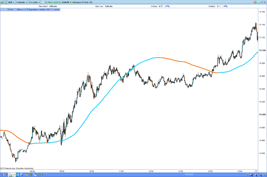
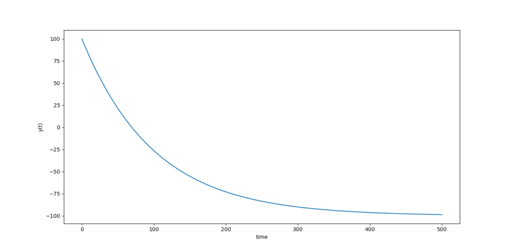
The two following charts show a linear regression and a smoothed linear regression:
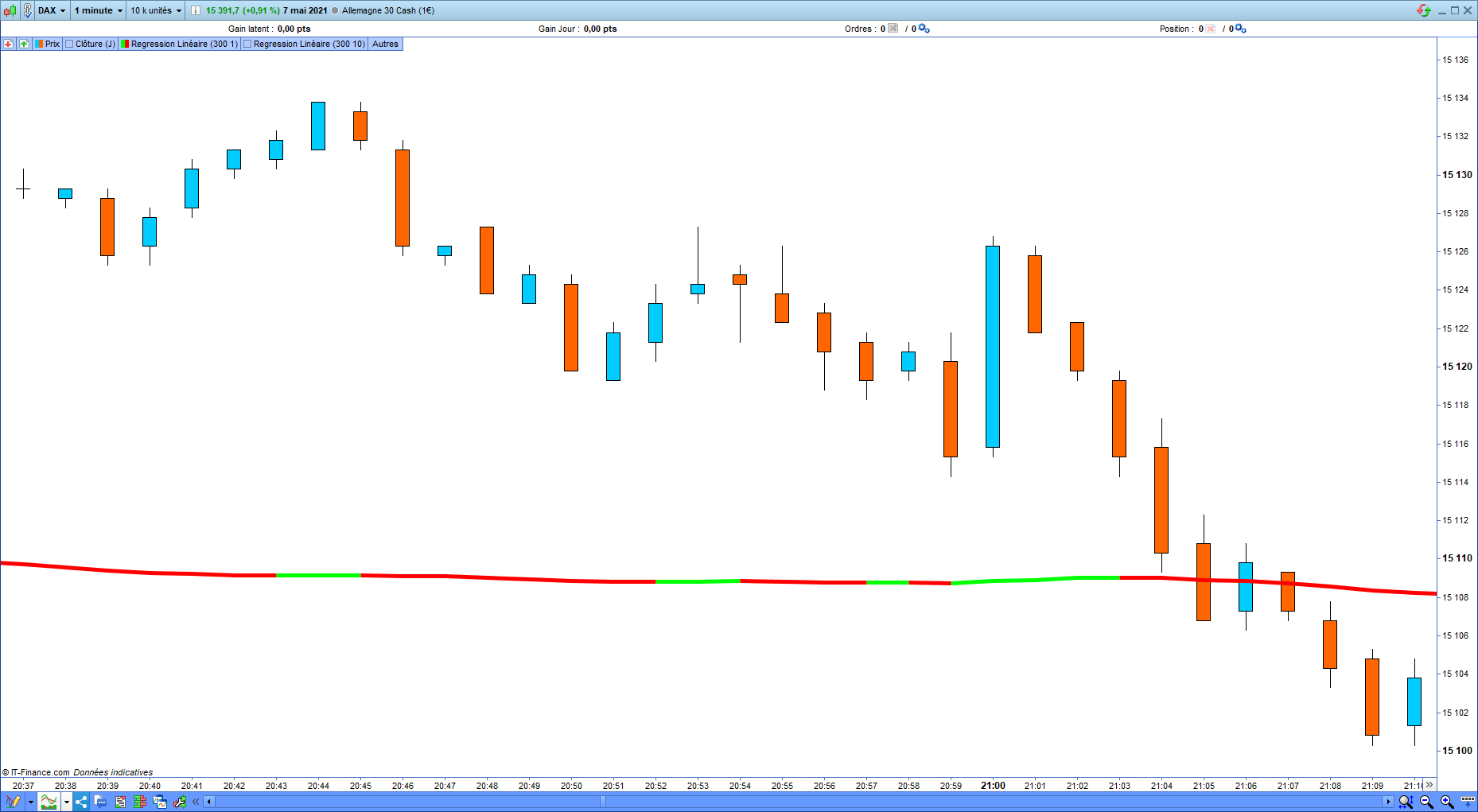
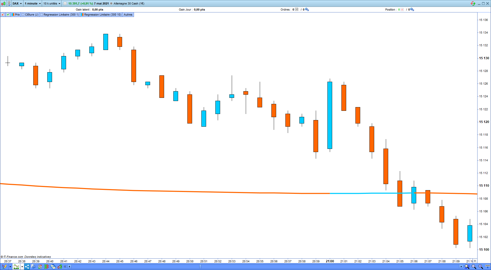
You can see several variations of the linear regression slope on the not-smoothed linear regression (the first picture). These changes will generate a lot of false signals in the trading system. In the second chart, the linear regression indicator is smoothed over ten periods. You can see that there is only one false signal. However, as I already said, smoothing a technical indicator may reduce some false signals, but avoiding them is impossible.
II. Backtest and optimization of a trading system
Optimizing an automated trading system is the most complex and delicate part of trading system design. There are a lot of concepts to know and apply. I will not present how I choose a value because that is not the subject of this post.
I described the main optimization models in my book, which you can find here: https://artificall.com/product/automated-trading-thanks-to-prorealtime-ebook/
The Prorealtime optimizer of the variables
Now, I will show you how to use the optimizer of the variables available on the Prorealtime platform. That will allow you to test a range of values on a variable and see the behavior of your strategy depending on each value.
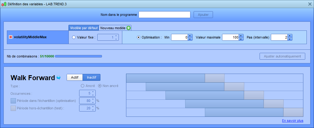
Run an optimization of the variables
For this example, I will run the optimizer on the “volatilityMiddleMax” variable from ‘0’ until ‘100’ with a step of ‘2’.

After that, you have to restart the backtest and look at the behavior of the strategy depending on the evolution of the “volatilityMiddleMax” variable.
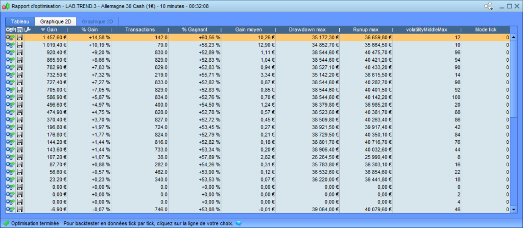
Understand the optimizer of the variables’ result
After launching the optimizer of the variables, a table will appear, including the result of each tested value:
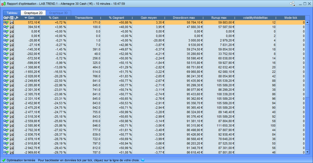
You can see that the strategy only gave a return with a standard deviation lower than 12 calculated on 100 periods. You can also note that the more the value of the “volatilityMiddleMax” variable increases, the more the number of entry openings increases.
The optimizer of the variables of Prorealtime allows printing the backtest result in graph form. It is possible to print the evolution of different metrics like the performance, the drawdown, the runup, the number of winning entries, or the number of opening entries.
Number of entries opened by the trading system
The following graph shows the evolution of the number of opening entries by the trading systems depending on the value of the “volatilityMiddleMax” variable.
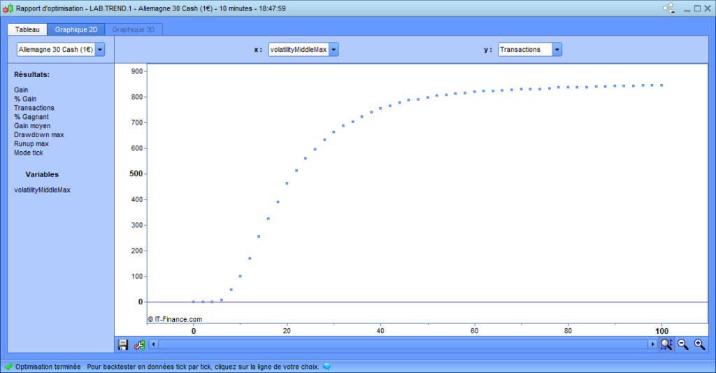
The graph above shows the evolution of the number of entry openings depending on the increase of the “volatilityMiddleMax” value. That is logical because the more the value of the “volatilityMiddleMax” variable increases, the more the trading system tolerates high volatility before opening an entry.
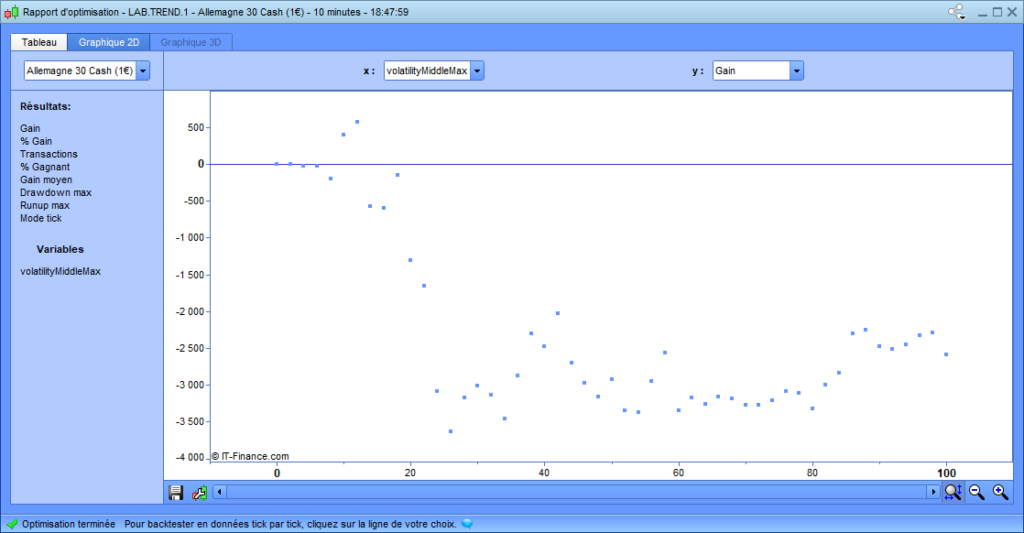
Over-trading consequences
The following graph shows the evolution of the equity curve depending on the evolution of the number of entries opened by the trading system. Remember that the number of entries is highly influenced by the value of the “volatilityMiddleMax” variable. You can see a negative correlation between the number of entry openings and the equity curve. That means the more the number of entries increases, the more the return decreases. Two possible reasons could explain this negative correlation.
1. The transaction cost
The first reason for explaining the negative correlation between the number of entries and the equity curve could be the invoiced fees for each transaction. The more the number of entry openings increases, the more transaction cost increases. If the trading system tolerates too much volatility, it will open many entries. This is equivalent to overtrading.
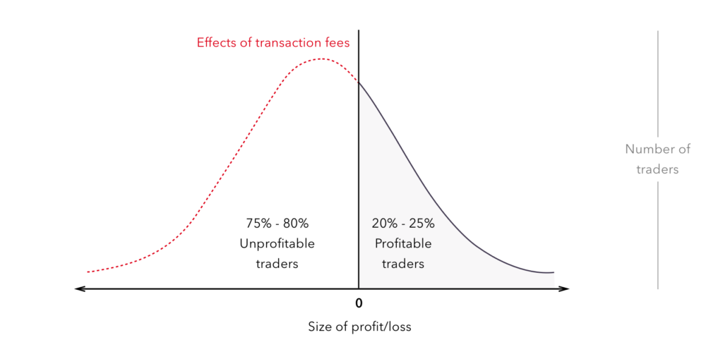
The picture below shows that the transaction cost move decreases the probability of being a winner in the financial market. That is why I prefer to operate only in the thin market. That is to say, I prefer to operate the main index like the Dax index because the « spread/ profit expecting » ratio is the most attractive.
2. Expecting gain by entry
The second reason that could explain the negative correlation between the number of entries and the equity curve is that it is difficult enough to find a lot of good opportunities on the same day. After many tests, I noted that finding more than two daily opportunities for a day-trader automated system is difficult.
This picture shows the evolution of expecting gain by entry by day. The expected gain by entry decreases while the number of entry openings increases daily until it becomes negative:
Limit the number of entries by day
As you can see, limiting the number of entries by day in your trading system is important. I integrated this functionality into the Automated trading system template I propose on my website. This template allows you to define the maximum number of entries by day in your trading system. That will enable you to secure your profits and avoid the risk of a series of losses if the market does not go in your trend.
Now, we have to ensure the profit potential of this little automated strategy thanks to the MFE and the MAE.
Validate the potential profit of a trading strategy
After the first backtest of your automated trading system, you must ensure that the profit potential exceeds the risk of loss. To validate the gain potential of a trading strategy, you can use the MFE and the MAE. I will present these two metrics to you in the following paragraph.
Definition of the MFE and the MAE
MFE means “Max Favourable Exécution”. That corresponds to the highest latent profit reached after an entry opening. MAE means “Max aversion Exécution”. That corresponds to the highest latent loss after an entry opening. We will use these two metrics to evaluate the profit potential of a trading strategy.
Measure the profit potential of a trading strategy
Calculating the MFE/MAE ratio of an entry point or a trading strategy allows one to estimate its potential gains. The MFE/MAE ratio should be strictly greater than 1 to give a potential return. In this case, the highest-reached point is greater than the lowest-reached point after the entry opening.
If the MFE/MAE ratio of a long trading strategy is lower than 1, then that would mean that the tested entries would give a better return to sellshort these entries. And reversely, if the MFE/MAE ratio of a short trading strategy is lower than 1, that would mean that the tested entries would give a better return buy these entries.
In reality, the MFE/MAE ratio proposed on the Prorealtime platform represents the average of the highest and lowest points. Thus, when the average MFE exceeds the average MAE, the market tends to go higher after openings more often than lower. However, be careful because the used averages are arithmetic averages. The arithmetic average is affected by the extreme values. Thus, you should check if a significant event like the coronavirus crash has heavily impacted your backtest’s highest or lowest point.
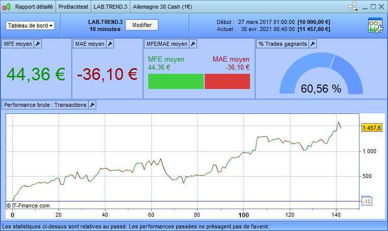
Potential profits of this automated trading strategy
Now, you have to verify if the chosen technical indicators for this little automated trend-following strategy are efficient. You must calculate the average MFE / average MAE ratio obtained during the backtesting.
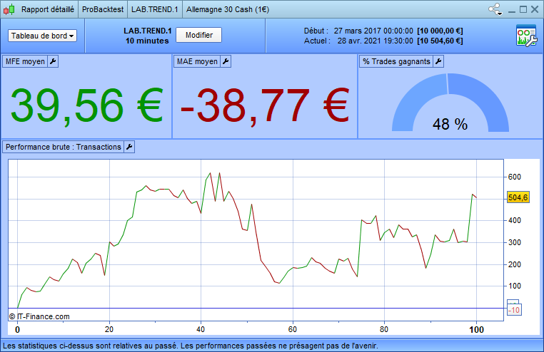
This is the result of the previous backtest, including the MFE and the MAE:
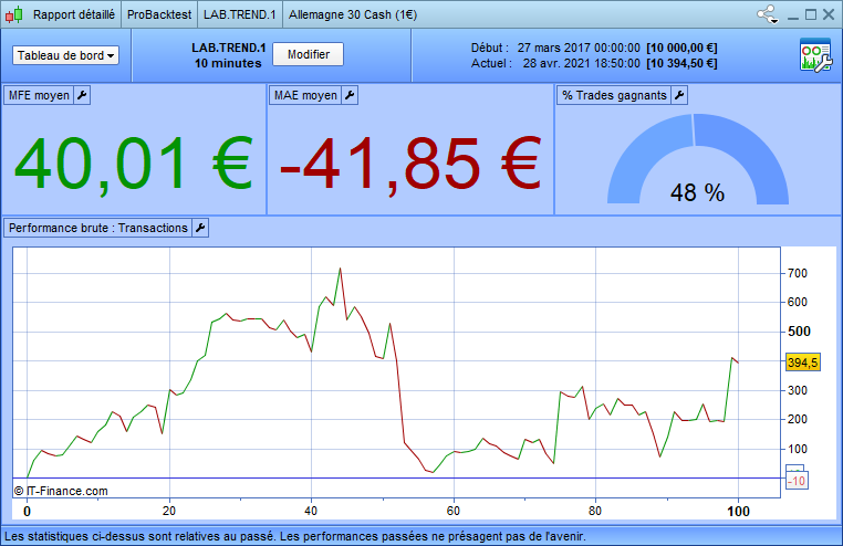
The obtained result is not unusual because the MFE/MAE ratio is lower than 1, and the success rate of the strategy is lower than 50%. Even if this trading system shows a positive return, this result is too poor to be run on a real trading account. You will have to improve this trading strategy by adding some functionalities. Let us implement a stop loss and a target to see the result.
III. Addition of a stop loss and target to the strategy
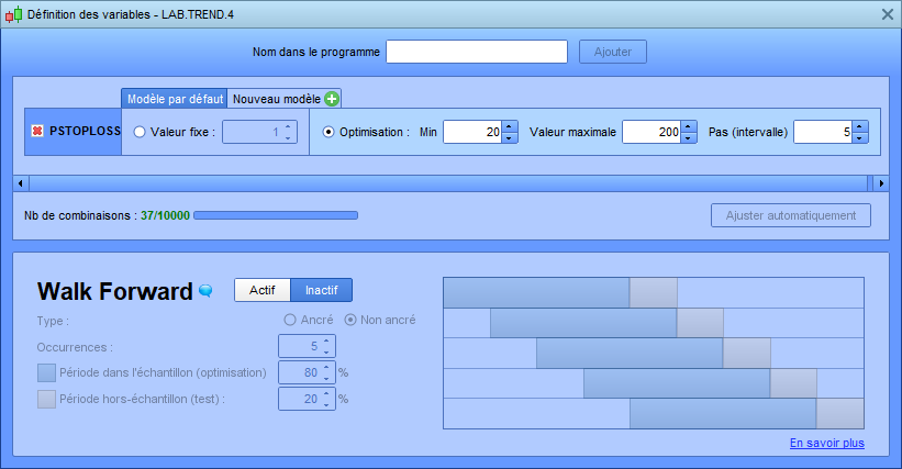
I will add a stop loss and a target in the previous source code. Their value will be static, and the target value will be two times the stop loss value for risk-reward reasons. I want to make the expected gain two times the risk of loss. The “PSTOPLOSS” variable will be used as a bench to define the stop loss and calculate the target. Now, you can try to optimize the stop loss and target position:
PSTOPLOSS = X
PTARGET = PSTOPLOSS * 2

SET STOP pLOSS PSTOPLOSS
SET TARGET pPROFIT PTARGET
Optimization of the stop loss and target
To optimize the stop loss and target position, you have to rerun the optimizer of the variables.
Run the optimizer of the variables on the stop loss and the target
The advantage to having defined a variable (PSTOPLOSS) from which the stop loss and target are calculated is that there is one alone variable to optimize. That represents a considerable time saved because the complexity of the backtest is reduced. You will run the optimizer of the variables on the “PSTOPLOSS” variable, with a range of values from 10 to 200 points. In this way, you will observe the evolution of the gain curve depending on the stop loss and target position.
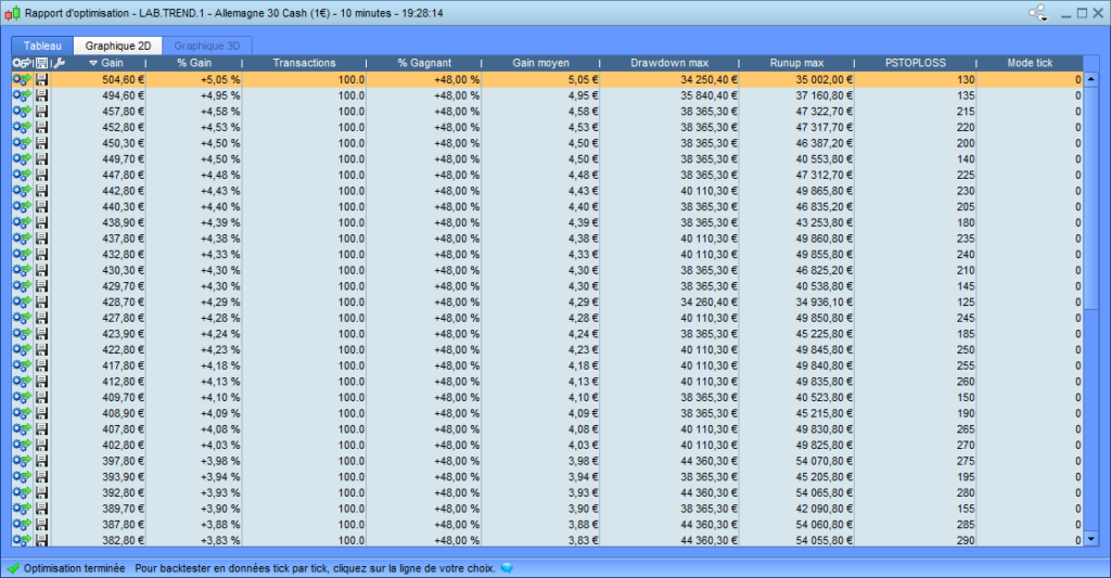
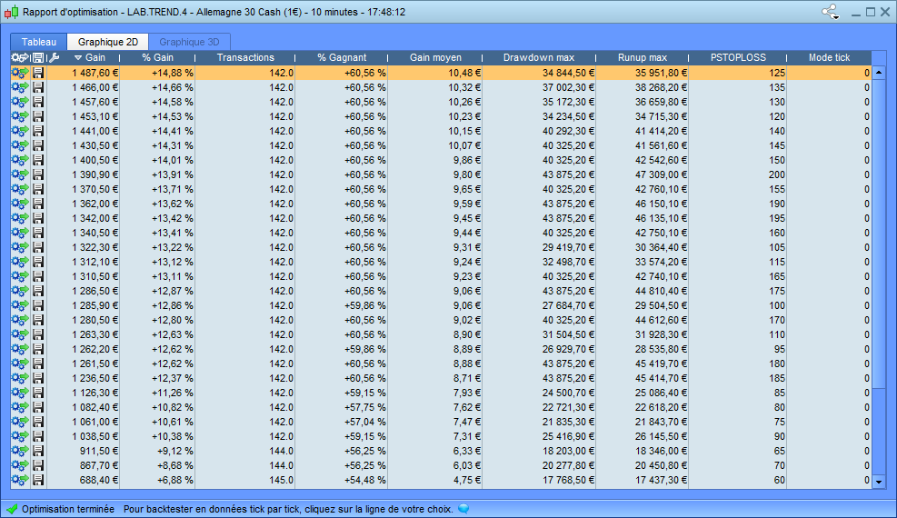
The optimization result shows that the most optimized value of the PSTOPLOSS variable would be 130 points. Since the target value is two times the stop-loss value, it is 260 points. Be careful because these values may be over-fitted. We will see that later.
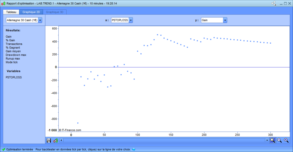
Equity curve evolution depends on stop loss and target
This is the evolution of the gain curve depending on the stop loss and target values:
Source code of the trend following system with a stop loss and target
This is the source code of this little trend following the trading system :
DEFPARAM CUMULATEORDERS = false
DEFPARAM FLATBEFORE = 090000
DEFPARAM FLATAFTER = 213000

// MARKET TREND USING LINEAR REGRESSION SLOPE
DRL300 = average[10](LinearRegression[300])
slope300 = DRL300[0] - DRL300[1]

conditionTrend = slope300 > 0

// VOLATILITY DETECTION
volatilityMiddleMax = 12
volatilityMid = STD[300] (close)

conditionVolatility = volatilityMid < volatilityMiddleMax

// Open a long entry
IF NOT LongOnMarket AND conditionTrend AND conditionVolatility THEN

	PSTOPLOSS = 130
	PTARGET = PSTOPLOSS * 2

	SET STOP pLOSS PSTOPLOSS
	SET TARGET pPROFIT PTARGET

	BUY 1 CONTRACT AT MARKET

ENDIF
Validation of the profit potential with a stop loss and target
To validate the impact of the stop loss and target addition on the previous trading strategy, you have again to check the MFE/MAE ratio:
This time, the MFE/MAE ratio is greater than 1 because it equals 1.02 (39.56/38.77=1.02). That means that integrating a stop loss and a target has improved the profit potential of the strategy. However, the success rate of the strategy stays the same.
IV. Find an entry point
The weakness of the previous trading system is that it opens an entry when the market becomes bullish and a few volatile but without real entry points. You could improve this trading system by implementing a set of technical indicators giving an entry point.
How to find a set of technical indicators?
There are a large number of technical indicators classified by category. There are four main technical indicator categories used in trading. There are trend, momentum, volatility, and volume indicators. Most of the time, the indicators from the same category are correlated.
This is the table including the leading technical indicators:
| Trend | Momentum | Volatility | Volume |
|---|---|---|---|
| Moving averages Exponential moving average (EMA) Moving average convergence divergence (MACD) Parabolic stop and reverse (Parabolic SAR) Linear regression Polynomial regression | Stochastic momentum Index (SMI) Commodity channel index (CCI) Relative strength index (RSI) | Bollinger bands Average true range Standard deviation Standard error | Volume Chaikin oscillator Onbalance volume (OBV) Volume rate of change |
Finding a good set of technical indicators in a trading system is often a long, hard process. That is why I use decision trees to test a combination of technical indicators quickly.
How to use a decision tree to find an entry point?
Decision trees are a fast and efficient way to discover a technical configuration that provides an arbitrage opportunity in the financial market. I explained how to use decision très using Prorealtime in this post: https://artificall.com/prorealtime/find-a-trading-strategy-on-prorealtime/
To find an entry point, I will select a set of technical indicators: RSI, MACD, and SMI. I don’t know if this set of indicators is the best choice, I just selected them for this example:
// Set of technical indicators to test
c1 = RSI[14] > 30
c2 = MACD [12,26,9] > 0
c3 = Stochastic[10,3](close) > 0
Source code using a decision tree
The following source code will test all the possible combinations of these three previous technical indicators:
DEFPARAM CUMULATEORDERS = false
DEFPARAM FLATBEFORE = 090000
DEFPARAM FLATAFTER = 213000

// MARKET TREND USING LINEAR REGRESSION SLOPE
DRL300 = average[10](LinearRegression[300])
slope300 = DRL300[0] - DRL300[1]

conditionTrend = slope300 > 0

// VOLATILITY DETECTION
volatilityMiddleMax = 12
volatilityMid = STD[100] (close)

conditionVolatility = volatilityMid < volatilityMiddleMax

// Set of technical indicators to test
c1 = RSI[14] > 30
c2 = MACD [12,26,9] > 0
c3 = Stochastic[10,3](close) > 0

// Brows the decision tree
IF cursor=1 THEN
	conditionDecisionTree = NOT c1 AND NOT c2 AND NOT c3
ENDIF

IF cursor=2 THEN
	conditionDecisionTree = NOT c1 AND NOT c2 AND c3
ENDIF

IF cursor=3 THEN
	conditionDecisionTree = NOT c1 AND c2 AND NOT c3
ENDIF

IF cursor=4 THEN
	conditionDecisionTree = NOT c1 AND c2 AND c3
ENDIF

IF cursor=5 THEN
	conditionDecisionTree = c1 AND NOT c2 AND NOT c3
ENDIF

IF cursor=6 THEN
	conditionDecisionTree = c1 AND NOT c2 AND c3
ENDIF

IF cursor=7 THEN
	conditionDecisionTree = c1 AND c2 AND NOT c3
ENDIF

IF cursor=8 THEN
	conditionDecisionTree = c1 AND c2 AND c3
ENDIF

// Open a long entry
IF NOT LongOnMarket AND conditionTrend AND conditionVolatility AND conditionDecisionTree THEN

	PSTOPLOSS = 130
	PTARGET = PSTOPLOSS * 2

	SET STOP pLOSS PSTOPLOSS
	SET TARGET pPROFIT PTARGET

	BUY 1 CONTRACT AT MARKET

ENDIF
Result of the decision tree
This is the result of the execution of the previous source code, testing all the combinations of the three technical indicators:
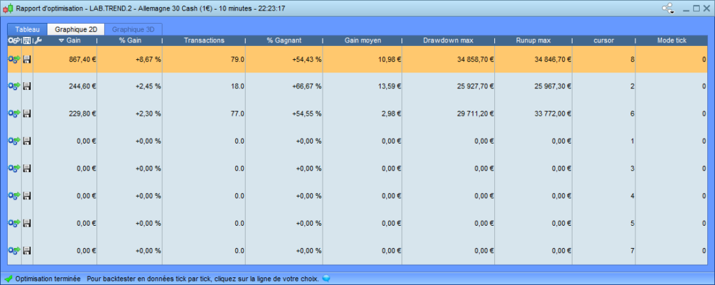
Regarding the result of the decision tree backtest, the combination giving the best return would be the eighth. This combination of conditions is the following:
c1 = RSI[14] > 30
c2 = MACD [12,26,9] > 0
c3 = Stochastic[10,3](close) > 0

IF cursor=8 THEN
	conditionDecisionTree = c1 AND c2 AND c3
ENDIF
The decision tree test shows us that an RSI[14] greater than 30, a MACD[12,26,9] greater than 0, and a Stochastic[10,3] greater than 0 improve the performance of this automated trend following strategy. Thus, you can implement these three technical indicators in the source code with the “c1 AND c2 AND c3” conditions.
Source code of trend following system with entry points
DEFPARAM CUMULATEORDERS = false
DEFPARAM FLATBEFORE = 090000
DEFPARAM FLATAFTER = 213000

// MARKET TREND USING LINEAR REGRESSION SLOPE
DRL300 = average[10](LinearRegression[300])
slope300 = DRL300[0] - DRL300[1]

conditionTrend = slope300 > 0

// VOLATILITY DETECTION
volatilityMiddleMax = 12

//volatilitySmall = STD[10] (close)
volatilityMid = STD[100] (close)

conditionVolatility = volatilityMid < volatilityMiddleMax

// Set of technical indicators
c1 = RSI[14] > 30
c2 = MACD [12,26,9] > 0
c3 = Stochastic[10,3](close) > 0

conditionDecisionTree = c1 AND c2 AND c3


// Open a long entry
IF NOT LongOnMarket AND conditionMarcheHaussier AND conditionVolatility AND conditionDecisionTree THEN

	PSTOPLOSS = 130
	PTARGET = PSTOPLOSS * 2

	SET STOP pLOSS PSTOPLOSS
	SET TARGET pPROFIT PTARGET

	BUY 1 CONTRACT AT MARKET

ENDIF
Validation of profit potential
As I did previously, I will verify the gain potential of this trading system thanks to the MFE/MAE ratio:
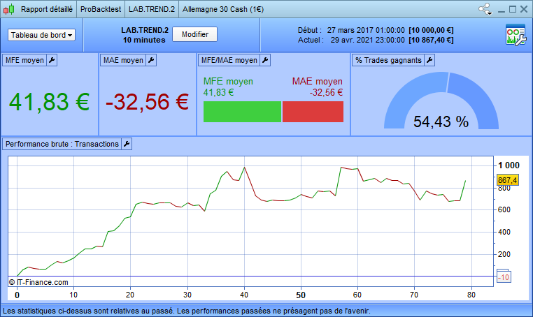
You can see that the MFE/MAE ratio has been considerably improved by adding the entry point. The MFE/MAE ratio now equals 1.28 (41.82/32.56=1.28). The success rate of the strategy rose to 54.43%, which is better than previously. The return passed from 501.6 points to 867.4 points. The entries decreased by 20%, strongly reducing this trading system’s risk exposure.
V. Global optimization of the trading strategy
Because you have added an entry point, you must relaunch a backtest on the variables to see the behavior of the trading system. You must optimize the trading system parameters again to check their correctness. Thus, you will test the stop loss and target position again and the maximum accepted volatility by the system.
Optimization of the stop loss and target
The position of the stop loss and the target significantly impact the result of the strategy. Thus, you should test again the “PSTOPLOSS” variable. This way, you will check if the initial value (130 points) is still efficient.
This is the result of the second optimization of the “PSTOPLOSS” variable:
The new value of the “PSTOPLOSS” variable giving the best return is 125 points, against the previously 130 points.
Validation of the profit potential after this new optimization
As I already made before, I will recheck the profit potential of this trading strategy using the MFE/MAE ratio.
Optimization of the volatility
Remember that the “volatilityMiddleMax” variable had the most impact on the number of entries opened by the trading system. Thus, you should rerun an optimization of this variable.
This is the result of the optimization of the maximum accepted standard deviation. Regarding the test, the value giving the best result for the “volatilityMiddleMax” variable is still 12:
Equity curve and entries of the trading system
This is the equity curve, including the entries opened by the trading system on the DAX index in a 10-minute time frame:
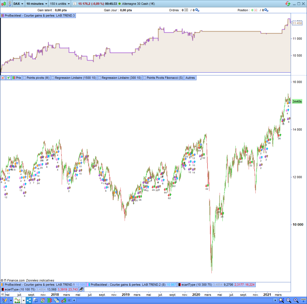
Interpretation of the trading system equity curve
From the beginning of the backtest until 2020, Marsh, the gain curve seems correlated with the DAX price evolution. We can say that the tracking error is probably low in this period. The number of entries in the trading system has fallen since 2020, Marsh. That comes from the excessive volatility in the market provoked by the coronavirus crash. The financial markets remained highly volatile throughout 2020. The trading system opened entries again at the beginning of 2021 because the market volatility was becoming normal.
Multi-dimensional optimization
The multi-dimensional optimization available on the Prorealtime platform consists of optimizing several variables simultaneously at the same time. That allows for observing the eventual interactions between the tested variables. Running a multidimensional optimization on two variables will allow you to see the gain curve evolution on a tridimensional graph. The two tested variables will represent the first dimensions, and the third will be the gain curve evolution.
Optimize the stop loss and target depending on the volatility
To optimize the stop loss and target position depending on the volatility, you can run the optimizer of the variables on the « volatilityMiddleMax » and « PSTOPLOSS » variables. However, the problem is that the number of possible combinations increases exponentially. Thus, you must reduce the range of tested values and increase the step. In this way, the number of possible combinations will be reduced.
To similarly test two variables using the optimizer of the variables, you have to add them as follows:
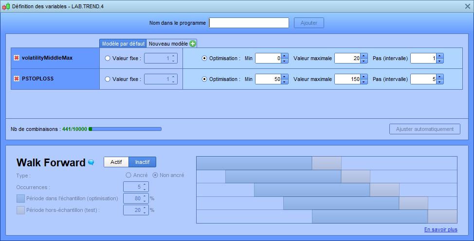
I reduced the range at [0; 20] for the « volatilityMiddleMax » variable with a step of 1, and I reduced the range at [50; 150] with a step of 5 for the « PSTOPLOSS » variable. The optimizer of the variables will have to test 21 * 20 combinations of values, that is, 441 combinations. The exécution time of the backtest would be reasonable.
3D Graph of the stop loss depending on the volatility optimization
It is possible to print the optimization graph in three dimensions. This way, you will observe the interaction between the stop loss and target position with the volatility.
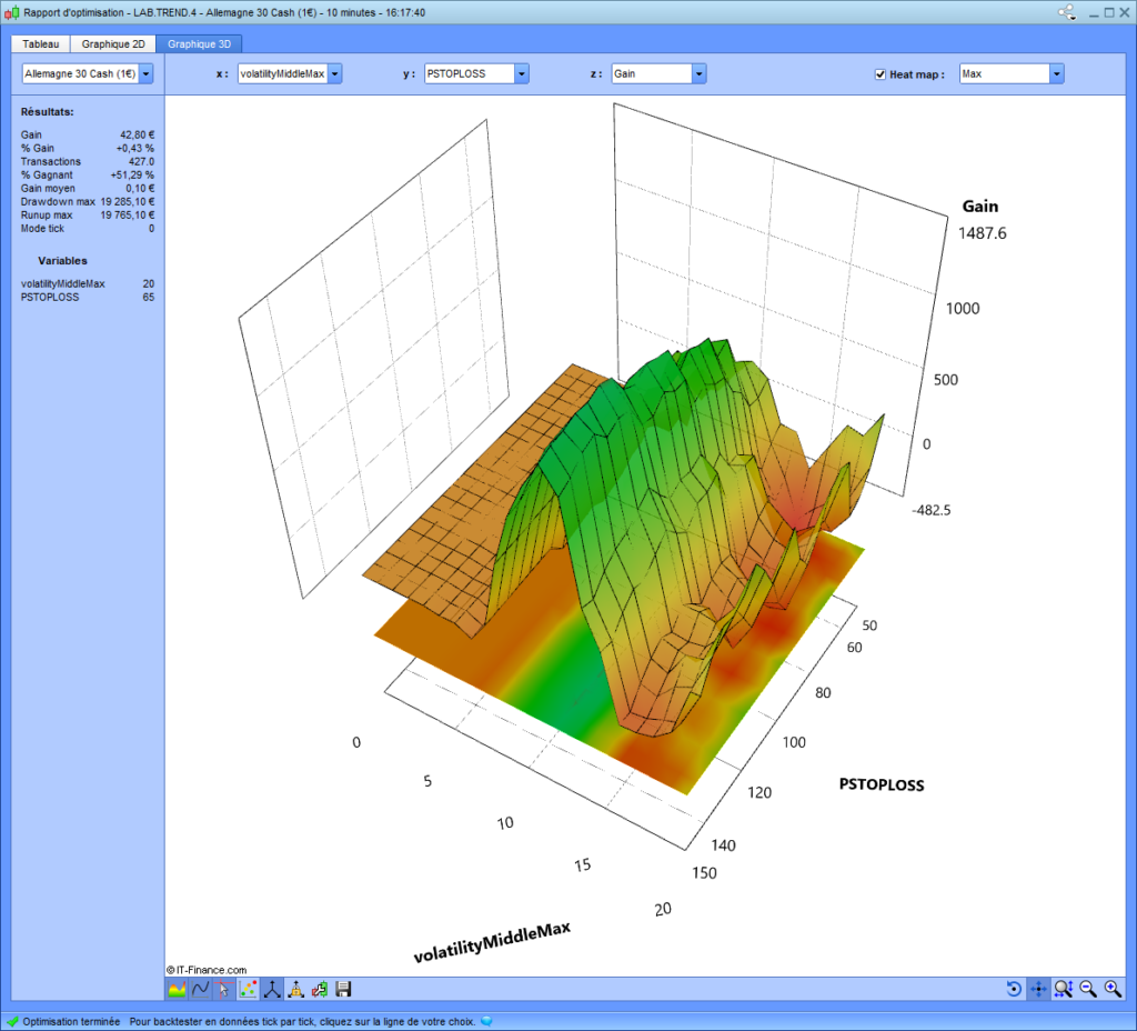
Interpretation of the stop loss depending on the volatility optimization
This test shows that the best return is obtained with a stop loss between 100 and 150 points when the maximum volatility is between 5 and 15 standard deviations. You can see that the trading system becomes looser for any stop-loss value when the maximum tolerated volatility is greater than 15 standard deviations. You can also see that the system loses when the stop-loss is lower than 50 points for any volatility value.
Automated trend following summary
Programing a trend-following system needs to follow several steps. You have to define the type of market that you want to operate by its trend, which can be bullish or bearish, and its volatility. Then, it would be interesting to find an entry point inside the chosen trend using some technical indicators.
I voluntarily simplified this trading strategy to facilitate your understanding of the different steps to build an automated trend-following system.
For example, defining the market trend would be preferable to using a trend indicator for several periods. That will also be the case with the definition of market volatility. The main difficulty is that a linear increase of used indicators provokes an exponential increase in the system’s complexity. The over-fitted risk will also increase exponentially depending on the linear growth of the used indicators.
Over-optimization risk management represents the largest part of creating a trading system. I won’t discuss this point in this post because that was not the subject. I already published some posts about the analysis of backtesting and over-optimization risks.
Range Breakout Indicator for Prorealtime [FREE]
The Range Breaker will help you seize the best trading opportunities. It detects range breakouts, which are often followed by explosive movements. Thanks to this indicator, you will never miss a breakout again.
The next Publication
In the next post, I will present how to use the PRT Bands indicator in a trading system working on Prorealtime.
If you have questions about this post, please let me know in the comments.
Thank you for reading.


Pingback: How to benefit from the pullbacks on the market?
Pingback: Find a trading strategy on ProRealTime
Pingback: The real success rate of Double Bottom
Pingback: The secret to winning in the future with a trader bot