
After evaluating your strategy’s robustness at first glance, your automated trading system must undergo a battery of stress tests to confirm its robustness.

In this post, I will show you how to test the robustness of an automated trading system using Prorealtime and Python.
Before launching your automated trading system on your real account, I will present the more important stress tests that you should make on Probacktest. I will also realize some Python simulations that would give you more visibility on the properties of your trading strategy.
Table of contents
- Spread increase simulations and tests
- Trigger stop loss by a single point
- Simulate the back to heads or tails
- The example of an asymmetrical strategy
- Back to heads or tails of an asymmetrical strategy
- The example of a symmetrical strategy
- Back to heads or tails of a symmetrical strategy
- Make your own simulations thanks to Python
- Example of successChanger function calling
- Conclusion about back to heads or tails test
- Series of losses and worst possible case
- Flash crash simulation
- Stress-tests summary
…
Spread increase simulations and tests
Simulating an increase in the spread is the first test I do to verify the robustness of a strategy. It is the easiest and fastest way to know if an automated trading strategy is over-fitted.
This stress test consists of gradually increasing the spread cost invoiced at each entry until the strategy’s performance becomes null or a few lose. This is my interpretation of the spread increase result:
- If your strategy generates loss after a few spread-increasing, that means your strategy is certainly over-fitted.
- If your strategy continues to win money after several spread increases, that may indicate that your strategy is under-fitted.
How to conduct this stress test?
Usually, I divide the spread-increasing test into two parts: first, I simulate the stress test thanks to a Python function, and next, I launch this stress test on Probacktest.
Python stress test simulation
I begin to simulate the consequences of the spread increase on my strategy. I use a Python function to proceed with this test. This first simulation helps me visualize the effect of spread increasing on a graph.
Probacktest stress test launching
Then, I launch a backtest on the Prorealtime platform, increasing the spread iteratively. After each iteration, I analyze all entries impacted by the rising spread, particularly entries that lost too quickly.
Simulation of spread increasing
I will begin by simulating the consequences of spread increasing on a strategy from its properties. By “properties” I mean the started capital, the success rate, the average gain, and the average loss.
The Python function takes in parameters for the strategy’s properties. In addition, the function integrates the spread and the number of entries into its parameters.
The function returns the simulation’s result in a matrix, which is then translated into a PNG image.
Source Code of the backtest Python function
# import of libraries
import random
import matplotlib.pyplot as plt

# instanciation of needed objects
rnd = random.Random()

# declaration of  backtest
def backtest(capital, successRate, gain, loss, spread, numberFlips):
	resultat = []
	trade = 0
	startupCapital = capital
	failureRate = 100 - successRate
	i = numberFlips

	while i > 0 and capital > 0:
		trade = rnd.choices([gain, loss], weights=(successRate, failureRate))
		capital = capital + trade[0] - spread
		resultat.append(capital)
		if capital <= 0:
			break
		i-=1

	plt.figure(figsize=(12,5))
	plt.axhline(startupCapital, color="gray")
	plt.plot(resultat)
	plt.show()
	plt.close()


# Example of backtest function calling
backtest(10000, 55, 28, -25, 1, 1000)
Now, I will explain how this function works, the used objects, its parameters, and the simulation algorithm.
Libraries called by backtest function
The “backtest” function calls two libraries: the Random library and the Matplotlib library.
Random
The Random library is necessary to generate random sequences. I use this library to create a sequence of winning and losing trades with a predefined probability.
To use this library, you need to instantiate a “Random” object in this way :
rnd = random.Random()
Matplotlib
The Matplotlib library is very famous and largely used in mathematical applications. We will use this library to create a chart from a NumPy matrix.
Parameters of the backtest function
The following parameters will allow us to create a personalized simulation :
| Parameter | Description |
| capital | Your started capital |
| successRate | Success rate in percent of your strategy |
| gain | Average gain in points of wining entries |
| loss | Average loss in points of losing entries |
| spread | Invoiced spread for each opened entry |
| numberFlips | Maximal number of entries that the function can open |
Algorithm of backtest function
The algorithm of the backtest function is pretty simple. The simulation continues while the capital is greater than zero.
WHILE CAPITAL > 0 DO
    SIMULATE AN ENTRY
    INTEGRATE THE RESULT IN THE CAPITAL
END-WHILE
Stages of the algorithm :
- The treatment running while capital greater than zero
- A trade is simulated at each iteration
- This trade creates profits or losses
- The result is integrated into capital
- The value of “capital” variable is added into the “resultat” matrix
Explanation of source code
I will explain to you the more important code lines of backtest function.
Generate a random entry:
The following code line will generate an aleatory trade thanks to the “choices” function of the “Random” library. This function is called from a Random object named “rnd”. This “rnd” object was created before we declared the backtest function.
trade = rnd.choices([gain, loss], weights=(successRate, failureRate))
This trade is generated with properties passed as “backtest” function parameters. The parameters are the average gain (gain), the average loss (loss), the success rate (successRate), and the failure rate (failureRate, deducted from success rate).
- If the trade wins, the variable “trade” will equal the average gain (gain).
- If the trade loses, the variable “trade” will equal the average loss (loss).
Recalculate the value of capital :
For each iteration, the capital value needs to be recalculated depending on the last simulated trade result (trade[0]). Of course, the spread (spread) must be deducted from this result.
capital = capital + trade[0] - spread
Feed the “resultat” matrix :
The new capital value must be added to the “resultat” matrix. The “resultat” matrix contains the successive evolution of capital following each simulation iteration.
resultat.append(capital)
Displaying the result :
At the end of processing, the chart was created from the « plt » object and printed the matrix “resultat”. The next code line will create an empty chart with a width of 12 and height of 5 thanks to “figure” function:
plt.figure(figsize=(12,5))
Personally, I decided to draw a horizontal line thanks to the “axhline” function which corresponds to started capital to visualize the drawdown.
plt.axhline(startupCapital, color="gray")
Finally, the graph is plotted with the “plot” function and printed with the “show” function.
plt.plot(resultat)
plt.show()
Simulation running with Python
Now, we can simulate the effect of spread increasing on a strategy. The properties of our strategy will be the following:
The started capital is $10,000, and the success rate will be 55%. The strategy will open and close 1000 entries, with an average gain of 28 points, an average loss of 25 points, and a spread of 1 point.
The “backtest” function needs to be called in the following way:
backtest(capital, success rate, average gain, average loss, spread, number of entries)
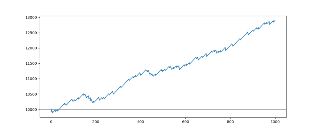
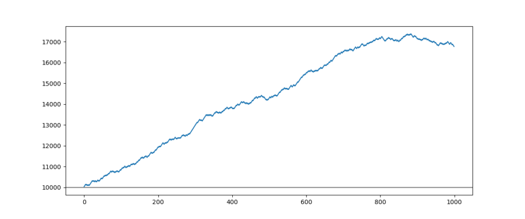
Simulation of the strategy with a spread of 1 point
# Calling up the function backtest
backtest(10000, 55, 28, -25, 1, 1000)
Result of simulation :
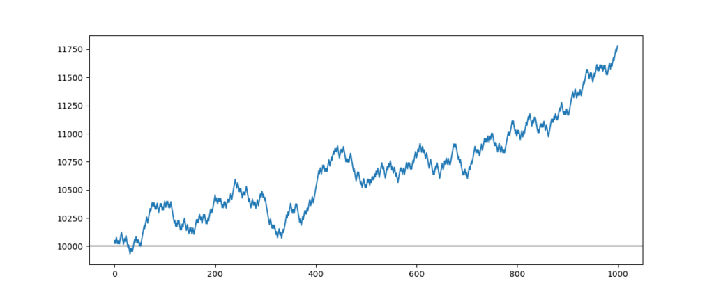
This strategy is globally profitable, performing 17.5% with 1000 entries. Let me show you what would happen if the spread rose to 2 points.
Simulation of the strategy with a spread of 2 points
# Calling up the function backtest
backtest(10000, 55, 28, -25, 2, 1000)
Result of simulation :
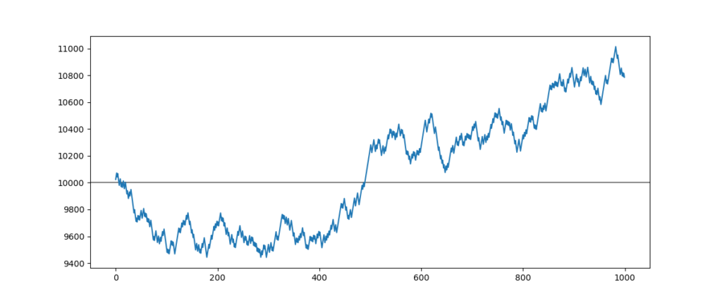
When the spread rises by 1 point, we can see an increase in volatility. In addition, we observe that the strategy’s performance was reduced to 7.5%, a 50% decrease.
Simulation of the strategy with a spread of 5 points
# Calling up the function backtest
backtest(10000, 55, 28, -25, 5, 1000)
Result of simulation :
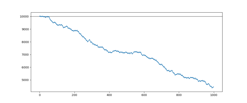
This strategy does not seem to endure an increasing spread. The strategy’s performance falls rashly and becomes lost when the spread reaches 5 points. The reason is that the difference between stop loss and target profit is too few. The difference was 4 points, then the spread was 5 points.
Simulation of spread increasing on Probacktest
From now on, we will have an idea of the spread increase’s consequences on a strategy’s performance. Thanks to Probacktest, we will submit this stress test on our strategy.
For that, we are simply going to increase the invoiced spread on the Probacktest interface and relaunch the backtest as below:
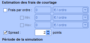
We will increase the invoiced spread for each transaction until the strategy performance becomes neutral or a few lose.
Over-fitted strategy behavior
I will begin to show you the reaction of an over-fitted strategy when the spread increases.
Strategy with a spread of 1 point
Strategy with a spread of 2 points
Strategy with a spread of 5 points
Interpretation of the result
Over-fitted strategies are highly sensitive to spread increasing. They become rapidly losing. Increasing the spread by 1 point on this strategy caused a fall in the success rate to 55%. This strategy became losing when the spread reached one-third of the average gain.
Under-fitted strategy behavior
Strategy with a spread of 1 point
Strategy with a spread of 2 points

Strategy with a spread of 5 points
Strategy with a spread of 20 points
Interpretation of the result
Under-fitted strategies are insensitive to the increasing spread. Their results are virtually not impacted. Even with an increase of 20 points corresponding to one-third of the average gain, the success rate is unchanged, and the strategy’s performance is still winning.
Summary of spread increase simulations and tests
About simulation
The increase in the spread provokes a strong negative impact on the performance.
This result is easy to understand. If the spread exceeds the difference between average gain and average loss, the strategy can not continue to win. The spread was 5 points, then the difference between average gain (28 pts) and average loss (25 pts) was 4 points : (28 – 25 = 4).
However, in reality, the variation of spread causes a variation in the success rate of an entry. We must launch a backtest on the Prorealtime platform to observe these variations.
About the backtest
Over-fitted strategies
Over-fitted strategies are very sensitives to the spread increasing. They become rapidly losing.
You could try to resolve this problem by widening your stop loss and target. If the widening provokes a fall in the success rate, the problem may come from your entry points.
In addition, if you decide to widen the stop loss and target, please ensure that the ratio stop loss/target remains unchanged.
Under-fitted strategies
Under-fitted strategies are few perhaps insensitive to spread increasing. Their success rate will be a few impacted by the spread.
You could resolve this problem by tightening your stop loss and target. As considered previously, if tightening your stop loss or target causes a fall in your success rate, then the problem might come from your entry points.
In the real world
In practice, the increase in spread seldom happens by chance. That happens during important events such as central bank announcements, market openings, or unexpected events.
I already noted that the spread tends to rise when the price of my entry is near its stop loss. This increase is often low and short duration but sufficient to touch the stop loss and close the position.
Thus, it is important to add a small gap at your stop loss positioning to maintain the same stop/target ratio.
Trigger stop loss by a single point
It is a variant of the previous method that allows you to measure the effect of stop-loss hunting on your strategy. In a backtest, your position will be conserved when the price moves towards a stop loss by a single point. By contrast, you may rest assured that your stop loss will be triggered when this situation happens in the real world.
This test consists of voluntarily triggering all stop loss when the price is nearer to it. To perform this test, you have two options: subtracting one point from the initial stop-loss or adding a conditional code line that closes an entry when the market price is too close to its stop-loss.
1. Subtract one point from the initial stop loss :
myStopLoss = 30 // your initial stop loss
SET STOP pLOSS myStopLoss – 1 // subtract one point
2. Trigger the closing of the entry when the market is too close:
Long position case :
IF low ≤ POSITIONPRICE - myStopLoss + 1 THEN
    SELL AT MARKET
END-IF
Short position case :
IF high ≥ POSITIONPRICE + myStopLoss - 1 THEN
    SELLSHORT AT MARKET
END-IF
These two alternative tests are important cause the spread-increasing test by the Probacktest interface is weak. Increasing the spread in this way provokes a tightening of the stop loss effectively and shifts the target. Thus, that introduces a negative bias in the final result.
Trigger stop loss summary
The worst way to optimize a strategy would be to optimize the stop loss and the target optimally, that is to say, by one point or less. You can be confident that your hyper-winning strategy on the backtest will be hyper-losing on your real account.
This test detects if the stop loss positioning is overfitted by one point. To be sure, reducing positioning by one point and observing the success rate is sufficient.
You should process the revert operation on the target, increasing its position by one point.
In an automated trading system, when a small variation in the value of a variable provokes a fall in performance, it is an “orphan value.” I will discuss “orphan value” in the next publication.
I will show you how to flush out the over-fitted variables, such as the stop loss, the target, or all other variables in decision-making. But before that, we will make an important simulation about the success rate of a strategy.
Simulate the back to heads or tails
The back-to-heads or tails test, as well as the spread increase test, is one of the most important tests in this chapter. This test simulates a strategy’s profitability and whether the success rate would drop to 50%.
For a strategy that continues to be profitable with a success rate of 50%, the average gains must be strictly greater than the average losses. It is also important the biggest gain must be greater than the biggest loss.
A strategy that continues to be profitable despite a success rate of 50% guarantees the security of your capital. That allows you to test a new strategy with fewer overall risks. That also protects you against a strategy becoming obsolete.
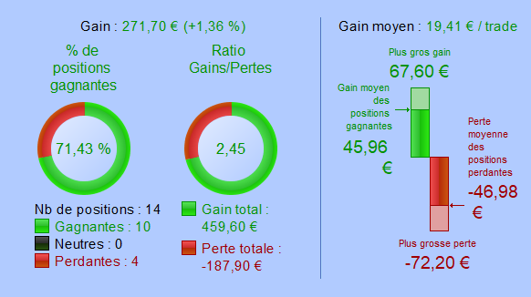
An example of an asymmetrical strategy
An asymmetrical strategy is a strategy for which the stop-loss position is far higher than the target position, and the success rate is high. Take the example of a strategy for which the stop-loss position is 30 points, the target position is 10 points, and the success rate is 85%. In this case, the stop loss is three times higher than the expected gains.
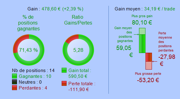
Hereafter the result of this asymmetrical strategy
On paper, this strategy appears very winning cause the printed performance is 28% of gains while 1000 entries.
If we zoom in on the result of this strategy, it should be noted that there are some big downfalls of the performance when there are losses:
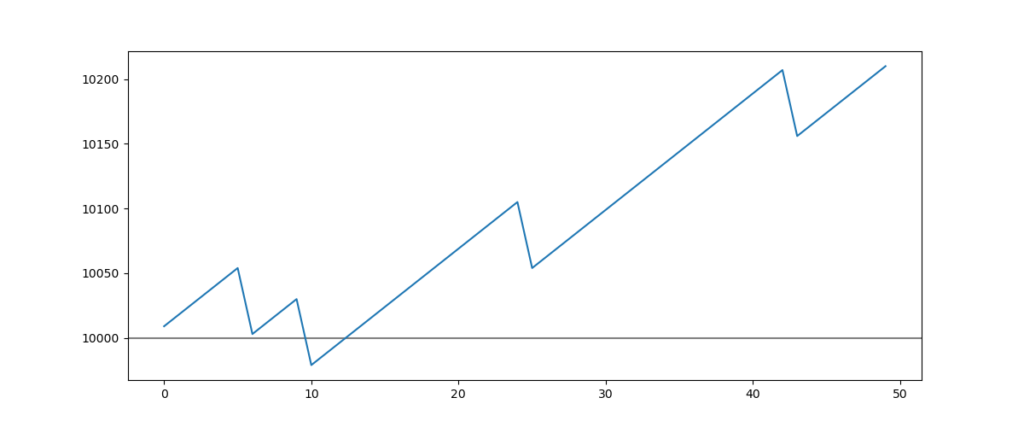
Now we are going to simulate the consequences on the performance and whether the success rate of this strategy would go down to 50%:
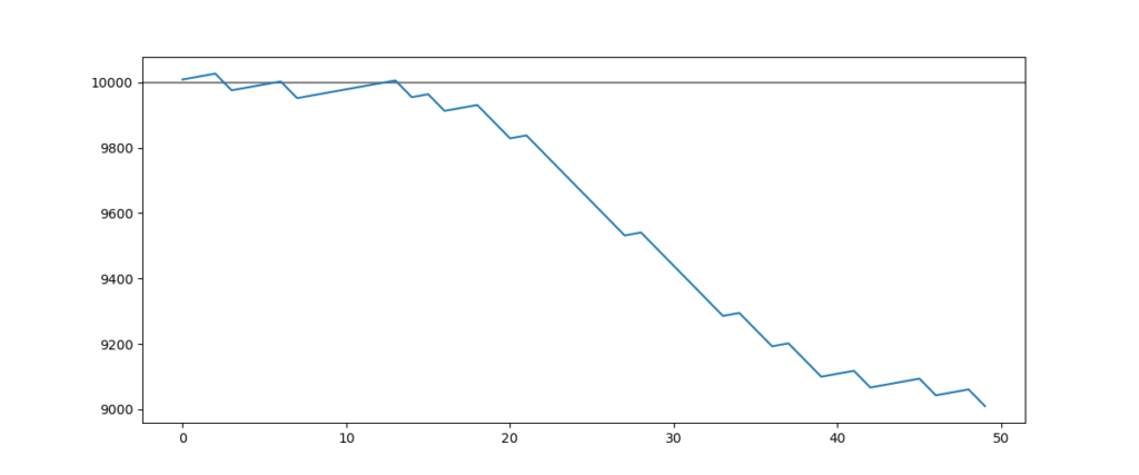
We can see that this strategy loses 10% of the stated capital (10000$) after only a little under 50 entries.
Back to heads or tails of an asymmetrical strategy
The most probable comportment of an over-fitted asymmetrical strategy at the time of its launching on the real account is the following:
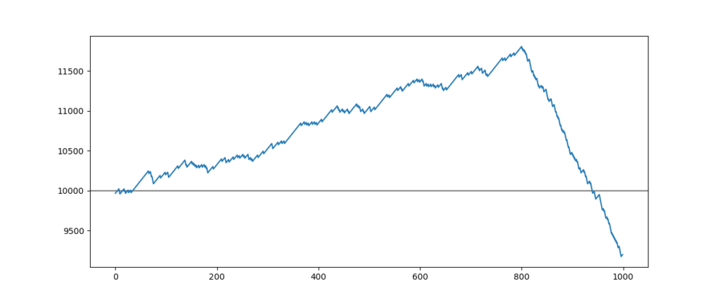
For this strategy, the stop loss position was 30 points, the target position was 10 points, and the success rate was 85%.
The 800 first entries represent the indicated performance, while the backtest then the 200 following entries correspond to the real account result.
The crash force comes from the imbalance in the gap between the average losses and gains. This strategy wins 10 when it loses 30.
An example of a symmetrical strategy
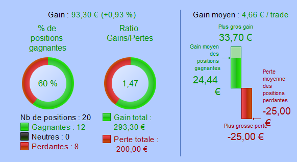
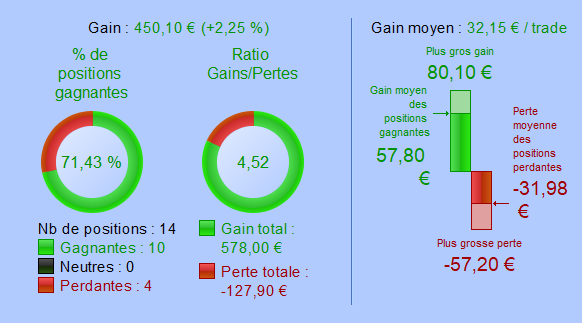
This time, we are going to test a symmetric strategy. That is, the success rate is slightly greater than 50%, and the average gain is slightly greater than the average loss. We will set 30 points for the target, 25 points for the stop loss, and 1 point for the spread. The strategy’s initial success rate will be 65%, and the started capital will be $10,000.
Hereafter the result of this symmetrical strategy
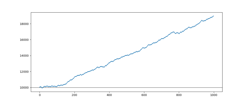
This strategy seems very winning, the printed performance is 80% of gains while 1000 entries.
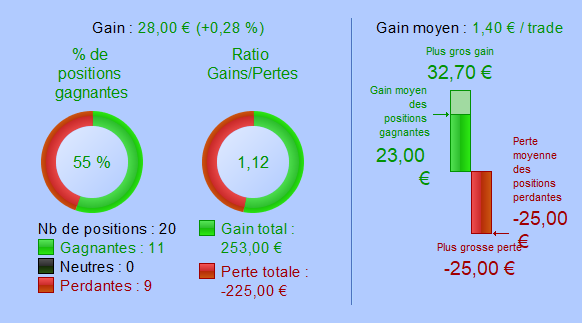
Now, we are going to simulate the consequences on the performance of whether the success rate of this strategy would go down to 50%:
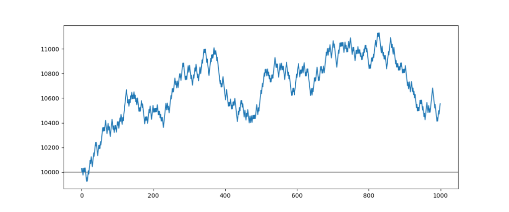
There is more volatility but the strategy continues to be a little winning with a profit of 5% with 1000 entries.
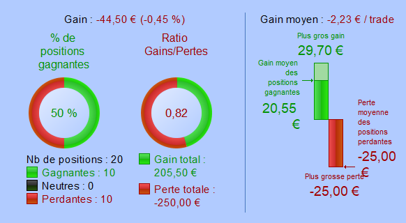
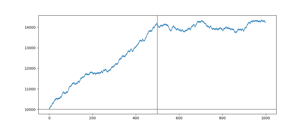
Back to heads or tails of a symmetrical strategy
The most probable comportment of an over-fitted symmetrical strategy at the time of its launching on the real account is the following:
The 800 first entries represent the indicated performance, while the backtest then the 200 following entries correspond to the real account result.
We can see that the strategy has difficulties continuing to give gains when the success rate is 50%, but it is still winning.
This approach defines an average gain greater than the average loss ensuring more security for your capital. Personally, I chose this configuration for all my automated trading systems.
Make your own simulations thanks to Python
I will show you the Python function I used in the previous examples. I named this function “successChanger” and I use it to measure and visualize the consequences of the back-to-heads or tails test on the performance of a strategy. This function derives from the “backtest” function, which I showed you in the “spread increase simulation” chapter.
successChanger function code source
def successChanger(capital, successRate1, successRate2, realSet, gain, loss, spread, numberFlips):
	resultat = []
	startedCapital = capital
	successRate = 0
	lossRate = 0

	i = numberFlips
	while i > 0 and capital > 0:
		if i > (numberFlips * realSet):
			successRate = successRate1
			lossRate = 100 - successRate1
		else:
			successRate = successRate2
			lossRate = 100 - successRate2

		a = rnd.choices([gain, loss], weights=(successRate, lossRate))

		capital = capital + a[0] - spread
		resultat.append(capital)
		if capital <= 0:
			break
		i-=1

	plt.figure(figsize=(12,5))
	plt.axhline(startedCapital, color="gray")
	plt.axvline(500, color="gray")

	plt.plot(resultat)
	plt.show()
	plt.close()
Call the function :
# Example of successChanger function calling
successChanger(10000, 65, 50, 0.5, 30, -25, 1, 1000)
Libraries called by backtest function
The “successChanger” function uses the same libraries as the “backtest” function, namely Random and Matplotlib.
Algorithm of successChanger function
The algorithm of the successChanger function is similar to that of the backtest function. The main difference is that the successChanger function divides the simulation into two parts: backtest and real. Each part will have its own success rate.
Pseudo-code of the algorithm :
WHILE CAPITAL > 0 DO
    IF FIRST-PART THEN
        SIMULATE AN ENTRY(successRate_1)
        INTEGRATE THE RESULT IN THE CAPITAL
    ELSE
        SIMULATE AN ENTRY(successRate_2)
        INTEGRATE THE RESULT IN THE CAPITAL
END-WHILE
Stages of the algorithm :
- The treatment running while capital greater than zero
- Verify if it is the first or the second part of the simulation
- Success rate assignment of the entry
- Entry simulation
- This entry generates a loss or a gain
- Integrate the result into the capital
- The capital variable is added to the “resultat” matrix
Parameters of successChanger function
The following parameters will allow us to create a personalized simulation:
| Parameter | Description |
| capital | Your started capital |
| successRate1 | First part success rate in percent of the strategy |
| successRate2 | Second part success rate in percent of the strategy |
| realSet | Second part duration of the simulation (ex : 0.2=20%; 0.5=50 %) |
| gain | Average gain in points of winning entries |
| loss | Average loss in points of losing entries |
| spread | Invoiced spread for each opened entry |
| numberFlips | Maximal number of entries that the function can open |
Example of successChanger function calling
This is a complete example of simulation thanks to the successChanger function:
successChanger(10000, 65, 50, 0.5, 30, -25, 1, 1000)
Parameter Analyses
Now I will describe each parameter passed in the previous function example:
| Parameter | Description |
| 10000 | The started capital is 10000$ |
| 65 | The success rate in the first part is of 65% |
| 50 | The success rate in the first part is of 50% |
| 0.5 | The two parts have the same size (500 vs 500) |
| 30 | The average gain is 30 points |
| -25 | The average loss is 25 points |
| 1 | The invoiced spread is 1 point |
| 1000 | 1000 entries will be simulated |
Result of the previous function calling
This simulation shows that the strategy gives 40% of profits while the success rate is 65%. When the success rate is 50%, this same strategy continues to be a little winning with a profit of 2.5%.
Conclusion about back the heads or tails test
The back-to-head or tails test is very important because the majority of trading strategies frozen in time are intended to become obsolete. When a trading strategy becomes obsolete, its success rate is around 50%.
A way to protect oneself against big losses is to guarantee that the average gains exceed the average losses.
To do so, the initialization of stop loss, target, and begin to gain securing should be defined in this way:
- The target should be two times greater than the stop loss. For example, if the stop loss is 30 points, the target should be at 60 points.
- The beginning of gain securing should be strictly greater than stop loss. Concretely, that means your automated trading system must begin to secure gains when the latent gain is greater than the stop loss level with an addition of some points. For example, if the stop loss is 30 points, the system should begin to secure the gain at 35 points. (I arbitrarily defined 5 points in addition to the example)
The symmetrical trading strategy I presented to you previously corresponds to this example. This style of trading respects the tactical approach that I personally practice. That means I must always win a little more points than I am ready to lose.
Even today, sometimes I put in production an automated trading system that promised me a very high success rate while backtesting but which finally wins one of the two calls on my real account.
Thanks to this approach, I can test new strategies with minimal risk.
Series of losses and worst possible case
Estimate the series of loss cost
Even a good strategy at a time can undergo a series of losses. This series of losses does not have a too great impact on your trading account. A series of ten losses must not be superior to 20% of your capital. That is equivalent to 2% of risk by entry. It is classical in money management.
Please be careful. When I talk about a series of losses, I refer to the biggest loss your automated trading system can do at a time. That means that if your system shows the greatest loss is 20 points and the stop loss is positioned at 50 points. You should consider 50 points as the biggest possible loss in your calculation.
It is important to do that cause if your strategy is under-fitted, it is possible that the stop loss is never reached while the backtest is launched on a too favorable part of the market. In this case, the printed average loss is invalid.
Worst possible case simulation
Simulate the worst possible case, which consists of computing how many consecutive losing entries are needed to lose the whole capital. As before, this calculation considers the stop loss and not the average loss.
This test consists of imagining what could happen if the stop loss was immediately reached after the opening of an entry.
In order to respect money management rules, an automated trading system must experience a minimum of 50 losses before losing all its capital. That also corresponds to 2% of risk by entry.
Knowing the maximum number of losses provoking a total capital loss is very important. This number will be a determinant for the future when you become an automated trading system manager.
Flash crash simulation
I fear the flash crash the most as a trader. Having an opened entry during a flash crash is the worst thing. The majority of traders are not ready for it, which relates to the previous idea about risk exposure and money management.
An automated trading system must survive a 20% market fall in under one minute. Thus, your automated trading system should never exceed a risk exposition of 500%, corresponding to leverage below or equal to 5.
USD/CHF Flash crash of 2015/01/15
The following flash crash occurred on 15 January 2015 after the Swiss National Bank re-evaluated the CHF 30% higher against the EUR.
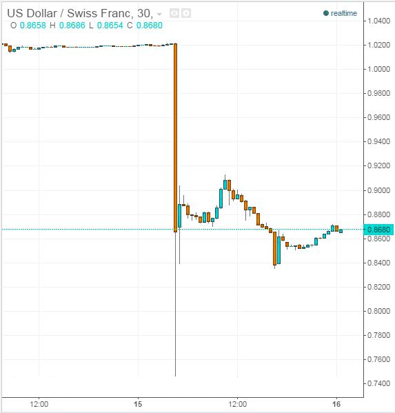
However, it is recommended that an automated trading system working like a day trader should never exceed 300% of marker exposure, and an automated trading system working like a swing trader should never exceed 100% of market exposure.
Stress-tests summary
The following is an overview of the stress tests chapter summarizing the main ideas to withhold that you could apply to your automated trading system :
- An automated trading system should accept a spread increase until ¼ of the average gain.
- The distance between the stop loss and the low point after the opening entry should always be more than 1 point.
- The average gain should always be greater than the average loss in the goal to continue to be a winner in the case of the success rate down to 50%.
- The market exposure should be reasonable; that is, it should be lower than 300% for a day trading strategy and lower than 100% for a swing trading strategy.
- While backtesting, the gain/loss ratio should be greater than 50%, which means your automated trading system should win at least slightly more often than one time in two.
- A series of 10 losses should not represent a loss of 20% of your capital.
- You should know how many losses provoke a total capital loss for each automated trading system running on your real account.
- An automated trading system must tolerate a fall in the market 20% would occur in under one minute without causing a total loss of capital.
In the next post, I will present to you a formidable stress test called “Stochastic modeling“. This test will give you the possibility to detect if your strategy is over-fitted with a high success rate.
For further information
Stress Testing, Investopedia
https://www.investopedia.com/terms/s/stresstesting.asp
Stress Testing for Trading Strategy Robustness by Michael R. Bryant
http://www.adaptrade.com/Newsletter/NL-StressTesting.htm
CrashMetrics
http://www.paulwilmott.com/crashm.htm
Range Breakout Indicator for Prorealtime
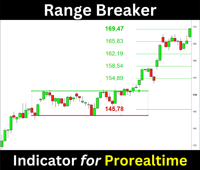
The Range Breaker will help you trade the Range Breakouts on Prorealtime. It displays the ranges, breakout signals, and target prices on your chart.