
Ultimately, achieving success with a trading bot in the past is relatively straightforward. Finding a winning strategy using three technical indicators and effective optimization in a backtest is relatively straightforward. The problem is that we want to win in the future. And here, things are more complicated.
In this post, I will present how to make money in the future using a trader bot. I will show you how to find the “fair optimization” that gives you the best chance to win in the future with a trader bot working on the Prorealtime platform.

Example of an automated trading strategy
To illustrate this point, I chose the example of a moving average crossing strategy. It is a straightforward trading strategy, but that will help you better understand the concept I will describe. You must run it on the DAX40 within a ’10-minute’ timeframe.
Description of the trading strategy
My chosen strategy will open a long entry when the 100-period moving average crosses over the 300-period moving average.
Source code of the entry openings
The following source code is runnable on the Prorealtime platform. It will open a long entry when the 100-period moving average crosses over the 300-period moving average. It will be active only during the cash market session, that is, from 09:00 until 21:30. All the opened entries will be automatically closed at 21:30 anyway.
// Strategy-test for the Dax 40 in a 10 minutes timeframe

DEFPARAM CUMULATEORDERS = false // only one trade in the same time
DEFPARAM FLATBEFORE = 090000 // avoide entry opening before this hour
DEFPARAM FLATAFTER = 213000 // close entry at this hour

//--------------------------------------------------------------------------
// ENTRY POINT
// Strategy of Moving average crossing
// MOVING AVERAGES
MM100 = average[100](close)
MM300 = average[300](close)

// Moving average crossing condition
conditionMovingAverage = MM100 CROSSES OVER MM300

//--------------------------------------------------------------------------
// OPEN A LONG ENTRY
IF NOT LongOnMarket AND conditionMovingAverage THEN

  PSTOPLOSS = //...
  PTARGET = //...

  SET STOP pLOSS PSTOPLOSS
  SET TARGET pPROFIT PTARGET

  BUY 1 CONTRACT AT MARKET

ENDIF
How to optimize an automated trading strategy?
The optimizer of the variables
The Prorealtime platform provides several optimization tools. It is notably the case of the “optimizer of the variables”. This tool will compute all the combinations of the values you want to test for a specific variable. Then, depending on the performance, it will sort the obtained results in ascending order.
Optimization sequence
I divided the test period into two equal samples for the purpose of this study. The first period will run from November 04, 2020, until July 13, 2021. The second period will run from July 13, 2021, until December 01, 2021. I will optimize the stop-loss and target during the first period. I will call this period “IS”, meaning “In the Sample”. Then I will check this optimization during the second period. I will call this period the “OOS” meaning “Out Of the Sample”.
| Starting date | Ending date | |
| In the Sample | 11/04/2020 | 07/13/2021 |
| Out Of the Sample | 07/13/2021 | 12/01/2021 |
I created this division to validate the efficiency of an optimization model. To validate this, I will optimize the strategy during the optimization period, then implement it in the IS, and subsequently run it on the OOS test period. If the performance between the two periods is significantly different, the model is probably inefficient.
Stop-loss and target optimization
Now, I will run the optimizer on the variables for the stop-loss and the target. First, I will optimize the stop-loss positioning and the target. I will select the stop-loss and target values that give the best return during the “In the Sample” period and verify this setting on the “Out Of the Sample” period.
Optimization of the stop-loss
To optimize the stop-loss, I need to execute the optimizer on the “PSTOPLOSS” variable. This variable sets the position of the stop-loss in points. For example, suppose the value of the PSTOPLOSS variable is 20. In that case, the trading system will place all the stop-losses 20 points under the position price immediately after the long entry opening.
Stop-loss optimization preparation
I commented out the code line allowing the PSTOPLOSS variable assignment because it is precisely the business of the optimizer. The optimizer of the variables will sequentially modify the value of the PSTOPLOSS variable.
I also removed the target code line from the source code to allow the optimizer to optimize the stop-loss independently.
The “FLATAFTER” parameter will close the entries at 21h30 anyway.
DEFPARAM CUMULATEORDERS = false // only one trade in the same time
DEFPARAM FLATBEFORE = 090000 // avoide entry opening before this hour
DEFPARAM FLATAFTER = 213000 // close entry at this hour

//--------------------------------------------------------------------------
// ENTRY POINT
// Strategy of Moving average crossing
// MOVING AVERAGES
MM100 = average[100](close)
MM300 = average[300](close)

// Moving average crossing condition
conditionMovingAverage = MM100 CROSSES OVER MM300

//--------------------------------------------------------------------------
// OPEN A LONG ENTRY
IF NOT LongOnMarket AND conditionMovingAverage THEN

  // PSTOPLOSS = //...
  // PTARGET = //...

  SET STOP pLOSS PSTOPLOSS
  // SET TARGET pPROFIT PTARGET

  BUY 1 CONTRACT AT MARKET

ENDIF
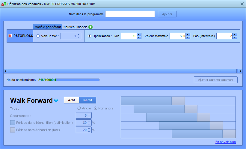
Configuration of the optimizer for the stop-loss
I set the minimum value to 10 points, the maximum value to 500 points, and a step size of 2 points. The optimizer will try 246 combinations of stop-losses, ranging from 10 to 500 in increments of two points. The optimizer will place a stop-loss at 10 points, then at 12 points, and then at 14 points, until it reaches 500, and relaunch the backtest each time.
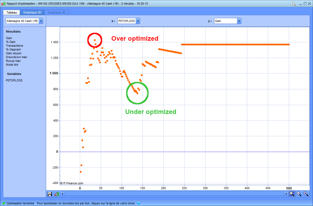
Result of the stop-loss optimization
The following graph shows the result of the stop-loss positioning optimization:
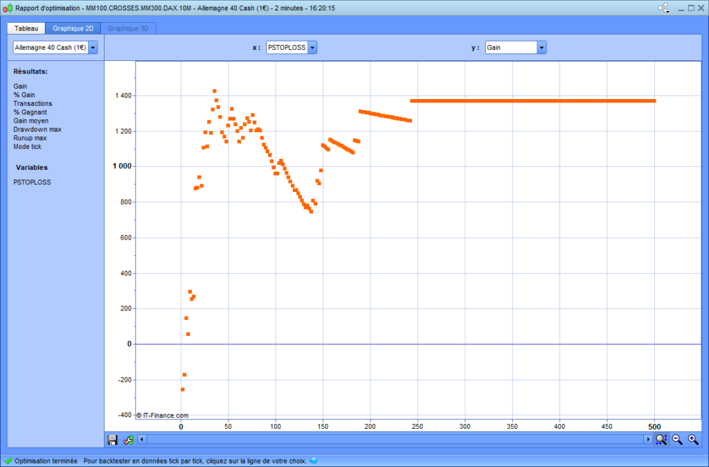
The abscissa axis represents the tested stop-loss values, and the ordinate axis represents the trading system’s performance depending on the stop-loss values. According to the previous outcome, a stop-loss at 36 points yields the best performance, resulting in a gain of 1,400 points during the test period. Thus, I naively set the PSTOPLOSS variable at 36 points in the trading strategy’s source code.
//--------------------------------------------------------------------------
// OPEN A LONG ENTRY
IF NOT LongOnMarket AND conditionMovingAverage THEN

  PSTOPLOSS = 36
  // PTARGET = //...

  SET STOP pLOSS PSTOPLOSS
  // SET TARGET pPROFIT PTARGET

  BUY 1 CONTRACT AT MARKET

ENDIF
Optimization of the target
The target optimization process is similar to the stop-loss process. I need to open the variable optimizer again and set the same test for the “PTARGET” variable.
Target optimization preparation
I commented that the code line allows the “PTARGET” variable because the optimizer will try several values. This time I keep the stop-loss code line with the value I found before, which is 36 points.
DEFPARAM CUMULATEORDERS = false // only one trade in the same time
DEFPARAM FLATBEFORE = 090000 // avoide entry opening before this hour
DEFPARAM FLATAFTER = 213000 // close entry at this hour

//--------------------------------------------------------------------------
// ENTRY POINT
// Strategy of Moving average crossing
// MOVING AVERAGES
MM100 = average[100](close)
MM300 = average[300](close)

// Moving average crossing condition
conditionMovingAverage = MM100 CROSSES OVER MM300

//--------------------------------------------------------------------------
// OPEN A LONG ENTRY
IF NOT LongOnMarket AND conditionMovingAverage THEN

  PSTOPLOSS = 36
  // PTARGET = //...

  SET STOP pLOSS PSTOPLOSS
  SET TARGET pPROFIT PTARGET

  BUY 1 CONTRACT AT MARKET

ENDIF
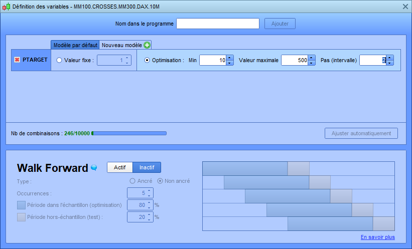
Configuration of the optimizer for the target
I defined the same configuration as the stop-loss optimization. I set the minimum value to 10 points, the maximum value to 500 points, and a step size of 2 points. The optimizer will try 246 combinations, ranging from 10 to 500 in increments of 2.
Result of the target optimization
The following graph shows the result of the target positioning optimization:
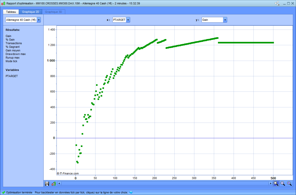
Regarding the result obtained by the variable optimizer on the test period, the best value of the target is 360 points. This value gives 1200 points of return. Thus, I will naively choose this value as the target in my trading strategy.
Overfitted configuration of the strategy
This is the code source of the trading strategy for which I naively optimized the stop-loss and target positioning. This configuration is probably overoptimized. I will implement this strategy during the IS period to see the results.
//--------------------------------------------------------------------------
// *** OVERFITTED STRATEGY EXAMPLE – DO NOT RUN ON A REAL ACCOUNT *** //
// * ACADEMICAL PURPOSE * //
// MM100.CROSSES.MM300.DAX.10M
// THIS STRATEGY MUST BE RUN ON THE DAX INDEX WITH A "10-minutes" TIMEFRAME
//--------------------------------------------------------------------------
DEFPARAM CUMULATEORDERS = false // only one trade in the same time
DEFPARAM FLATBEFORE = 090000 // avoide entry opening before this hour
DEFPARAM FLATAFTER = 213000 // close entry at this hour

//--------------------------------------------------------------------------
// ENTRY POINT
// Strategy of Moving average crossing
// MOVING AVERAGES
MM100=average[100](close)
MM300=average[300](close)

// Moving average crossing condition
conditionMovingAverage = MM100 CROSSES OVER MM300

//--------------------------------------------------------------------------
// OPEN A LONG ENTRY
IF NOT LongOnMarket AND conditionMovingAverage THEN

  // Overfitted setting
  PSTOPLOSS = 36
  PTARGET = 360

  SET STOP pLOSS PSTOPLOSS
  SET TARGET pPROFIT PTARGET

  BUY 1 CONTRACT AT MARKET

ENDIF
Result of the overfitted backtest
The optimization of the stop-loss and target that I proceeded with gave me a performance of 14.86% during the test period. This strategy’s success rate is 47.5%, the drawdown is four times lower than the runup, and the risk/reward ratio is 1.8. In other words, the result of this backtest does not show any lack or problem. It even looks perfectly acceptable!
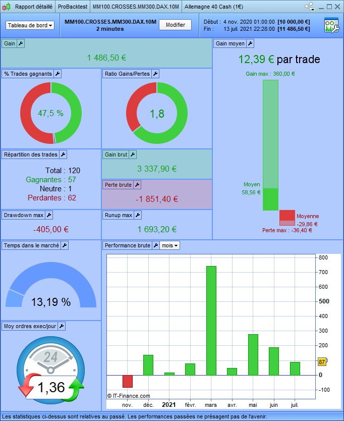
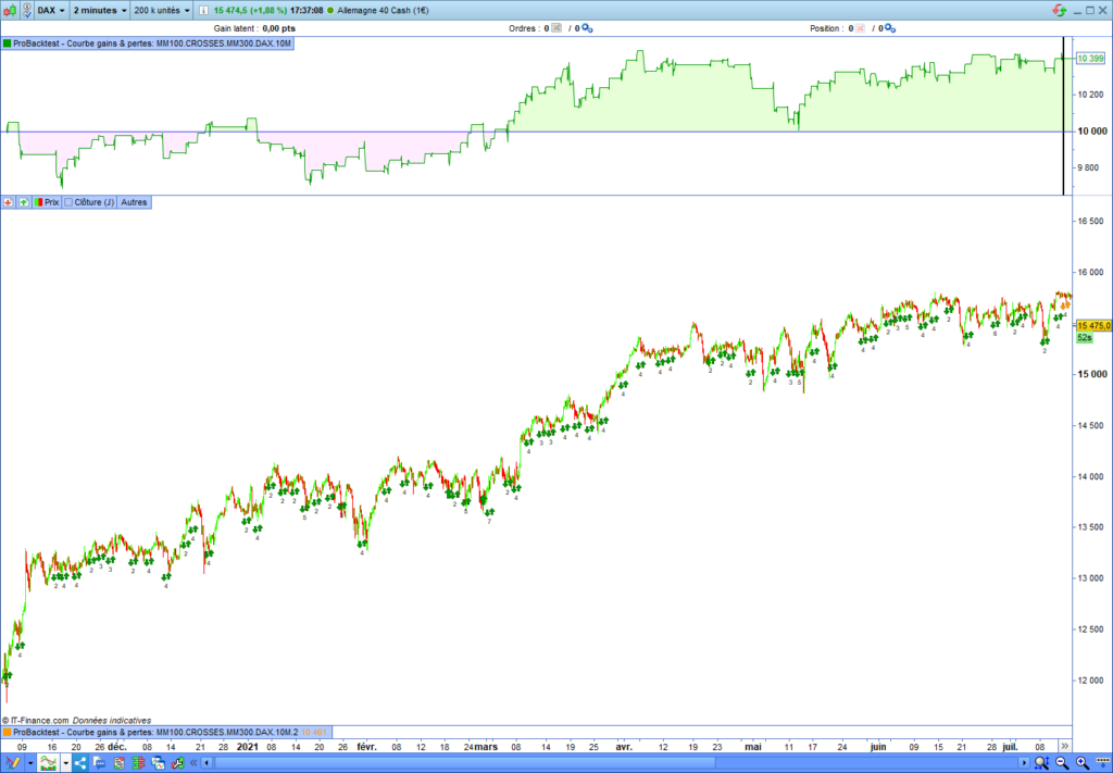
Equity curve of the overfitted backtest
The equity curve is imperfect and does not show an eventual overfitting problem. In short, this strategy is acceptable and looks ready to launch on a real trading account. [IRONY]
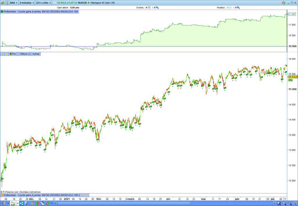
Now, I will compare the performance of this strategy during the IS period with the result during the OOS period.
Win in the past but lose in the future
I will run this fantastic trading strategy during the OOS period, specifically from July 13, 2021, to December 1, 2021, to validate its effectiveness.
Out of the sample validation
Here is the result of the strategy applied during the OOS period:
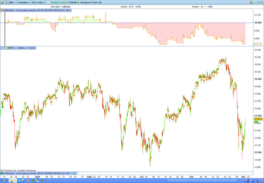
This wonderful trading system takes a trashing during the OOS period, to no one’s surprise. Unfortunately, it is the tragic fate of many trading systems.
How to find the fair optimization of a trading system?
When I started automated trading, I optimized my trading system incrementally, correcting losses one by one. I had fallen into the overfitting trap: I always won in the past but never in the future. It took a considerable amount of time and testing to understand how to succeed with a trading system in the future. The method I have found is counterintuitive, and you may find it difficult to accept.
I will explain how to process a trading strategy to find a fair optimization —that is, an optimization that will win in the future.
Deteriorate the equity curve of the backtest
Through numerous optimization tests of trading systems I conducted, I discovered an interesting phenomenon: the more a backtest has performed well in the past, the more it tends to underperform in the future.
Out of curiosity, I have had fun deteriorating the equity curve of the backtest and modifying the strategy’s configuration. What a surprise! This poor strategy in the past has become a winning one in the future. At this time, I realized the underfitting principle. I understood that it is better to voluntarily under-optimize a trading system instead of achieving the optimal one. (The correct optimization is supposed to be a point at the center between under-fitting and over-fitting)
Under-optimize the stop-loss and the target
I will voluntarily under-optimize the stop-loss and target positioning in my automated trading system. Later, I will compare the behavior of this trading bot between the in-sample (IS) and out-of-sample (OOS) periods. As a reminder, at the beginning of this study, I chose the stop-loss and target positioning that gave the best performance during the IS period. This configuration was lost during the OOS period.
To under-optimize the stop-loss and the target, I will choose the value for which the performance is two times lower than the best possible choice. The best performance of the stop-loss position gave a return of 1400 points. Thus, I will select the value for which the performance is nearest to 700 points. The best performance at the target position yielded a return of 1,200 points. Thus, I will select the value for which the performance is nearest to 600 points.
Under-optimize the stop-loss position
The following graph shows the optimizer result executed on the stop-loss variable. The over-optimized values are circled in red (at the top of the chart). They perform best during the in-sample (IS) period but lose in the out-of-sample (OOS) period. The under-optimized values are circled in green (at the bottom of the chart). Their performance during the IS backtest is two times lower than the over-optimized values:
I will choose one of the green-circled values and restart an OOS backtest to evaluate this trading system’s performance. However, I will also under-optimize the target before launching the backtest.
Under-optimize the target position
The following graph shows the optimizer result executed on the target variable. The over-optimized values are circled in red (at the top of the chart). They perform best during the in-sample (IS) period but lose in the out-of-sample (OOS) period. The under-optimized values are circled in green (at the bottom of the chart). Their performance during the IS backtest is two times lower than the over-optimized values:
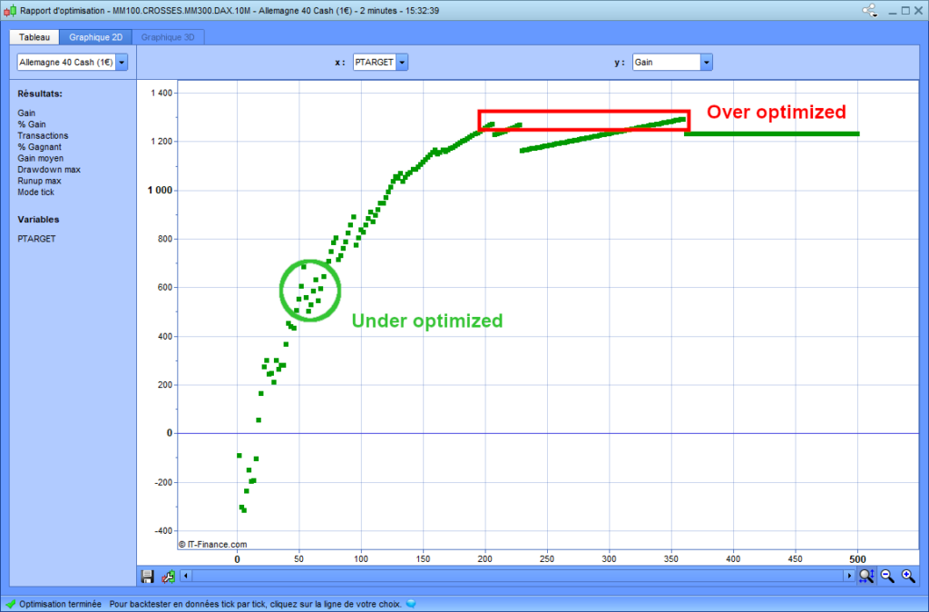
I will choose one of the green-circled values and restart an OOS backtest to evaluate this trading system’s performance.
Result of the under-optimized backtest
I will run a backtest with under-optimized values for the stop-loss and target. First, I will run the backtest on the IS period, and later, I will run the backtest on the IS period.
Source code of the under-fitted trading system
//--------------------------------------------------------------------------
// *** UNDER-OPTIMIZED STRATEGY *** //
// * ACADEMICAL PURPOSE * //
// MM100.CROSSES.MM300.DAX.10M
// AUTOR: Vivien Schmitt
// https://artificall.com
// DATE : 2021/12/01
// THIS STRATEGY MUST BE RUN ON THE DAX INDEX WITH A "10-minutes" TIMEFRAME
//--------------------------------------------------------------------------
DEFPARAM CUMULATEORDERS = false // only one trade in the same time
DEFPARAM FLATBEFORE = 090000 // avoide entry opening before this hour
DEFPARAM FLATAFTER = 213000 // close entry at this hour

//--------------------------------------------------------------------------
// ENTRY POINT
// Strategy of Moving average crossing
// MOVING AVERAGES
MM100=average[100](close)
MM300=average[300](close)

// Moving average crossing condition
conditionMovingAverage = MM100 CROSSES OVER MM300

//--------------------------------------------------------------------------
// OPEN A LONG ENTRY
IF NOT LongOnMarket AND conditionMovingAverage THEN

  // Overfitted setting
  PSTOPLOSS = 125
  PTARGET = 50

  SET STOP pLOSS PSTOPLOSS
  SET TARGET pPROFIT PTARGET

  BUY 1 CONTRACT AT MARKET

ENDIF
Performance of the under-optimized trading system
Here is the result of the trading system having an under-fitted stop-loss and target:
Validation of the optimization in the future
I will compare the performance of this trader robot between the in-sample (IS) and out-of-sample (OOS) periods. To facilitate this comparison, I will run a backtest on the in-sample (IS) period and another on the out-of-sample (OOS) period on the same chart.
IS and OOS performance comparison
The following chart compares the performance of the in-sample (IS) and out-of-sample (OOS) backtests. The IS backtest result is at the top, and the OOS result is below.
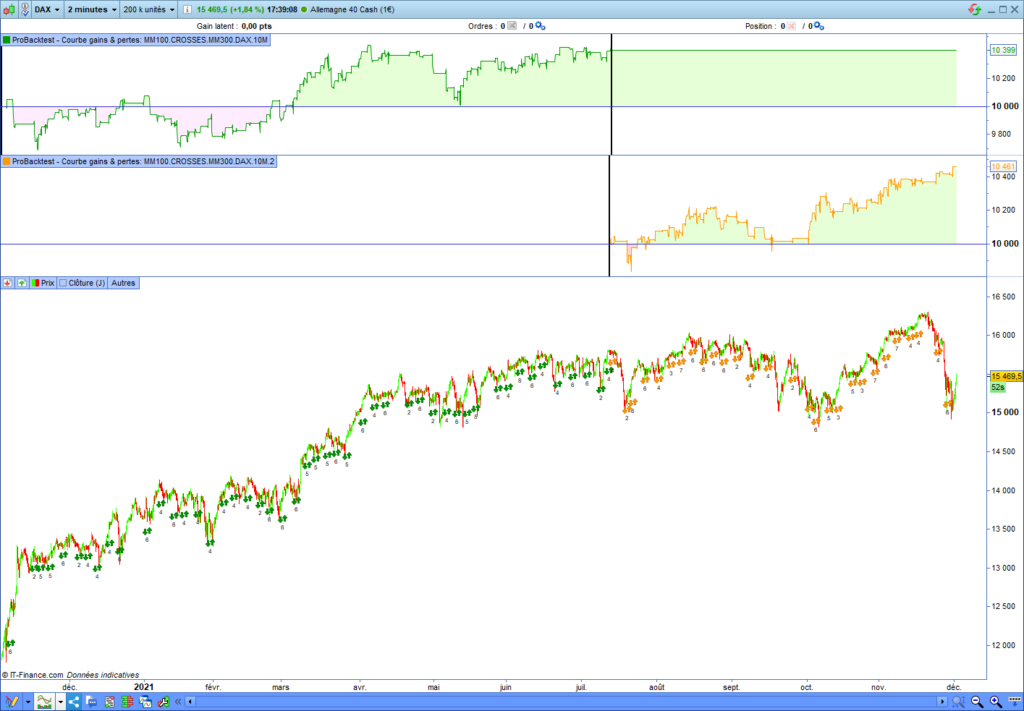
This time, the performance of the OOS backtest is positive. This under-optimized configuration will likely prevail in the future, confirming that an under-optimized trading system has a better chance of succeeding.
The limitations of the under-optimization model
As with all financial studies and all mathematical models, there are some shortcomings and limitations. I will present the most important to you.
Risk management in accordance
An under-optimized setting is always in keeping with your personal risk management rules. In this example, the final under-fitted values do not correspond with my risk management rules. The “target/stop-loss” ratio is lower than one (50/125<1), and I do not accept it. I respect the risk management rule saying that the target must be greater than the stop-loss. Thus, I can validate the previous trading system, nor run it on my real account.
Definition of an “under-optimized” value
The choice of under-optimized values is not perfectly established. In this example, I chose the values whose returns were two times lower than the highest performance during the IS backtest. This choice is relatively arbitrary and may not be the best choice.
What parameters need to be under-optimized?
I apply this model to the stop-loss and the target to support my arguments about the under-optimization duty. I cannot guarantee that it would be possible to underfit all the trading system parameters. And I don’t know if under-optimizing all the features would be profitable.
Optimization models
Several mathematical models, such as the WalkForward or Gradient Descent, enable the optimization of trading systems. As I write this, I have not found a perfect model that works each time. Each model has possibilities and limitations.
Under-optimization key points
- The more a trading system wins in the past, the more it risks losing in the future.
- An under-optimized trading system has a higher chance of winning in the future. It performs relatively poorly during the “In the Sample” period but gives a positive return during the “Out of the Sample” period.
- The definition of under-optimization is subjective. Sometimes, the choice can be difficult because of missing values.
- Unfortunately, perfect mathematical or machine learning models do not exist. They give only a probability of success.
Range Breakout Indicator for Prorealtime
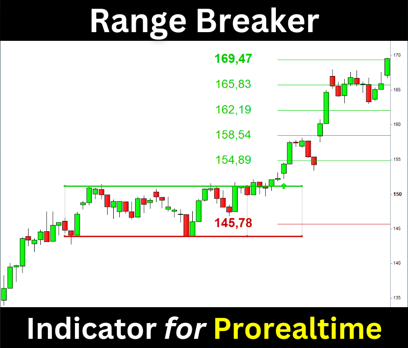
The Range Breaker will help you trade the Range Breakouts on Prorealtime. It displays the ranges, breakout signals, and target prices on your chart.
credit image: https://www.maxpixel.net/Mystery-Youth-Magic-Girl-The-Silence-Beauty-Ruda-4716922